TensorFlow TFRecord图形处理工具
在之前的文章里,我们介绍过Pillow这个强大的图形工具,跳转地址,今天我们再介绍一下 TensorFlow 是怎么预处理图像的。这二者有很多共通之处,下面我们就开始今天的图形之旅。
matplotlib是python上的一个2D绘图库,它可以在夸平台上边出很多高质量的图像。综旨就是让简单的事变得更简单,让复杂的事变得可能。我们可以用matplotlib生成 绘图、直方图、功率谱、柱状图、误差图、散点图等 。详细了解matplotlib,请点击这里
import matplotlib.pyplot as plt
import tensorflow as tf
import numpy as np

image_raw_data = tf.gfile.FastGFile("img/tiger/1351742906_31b427fb23.jpg",'rb').read()

with tf.Session() as sess:
    img_data = tf.image.decode_jpeg(image_raw_data)
    img_data.set_shape([1797, 2673, 3])
    print(img_data.get_shape())

    print img_data
    plt.imshow(img_data.eval())
    plt.show()

    img_data = tf.image.convert_image_dtype(img_data,dtype=tf.uint8)
    encode_img=tf.image.encode_jpeg(img_data)
    with tf.gfile.GFile("tfrecord/img_data.jpg","wb") as f:
    	f.write(encode_img.eval())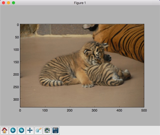
改变大小
缩放效果,参数method:
- ResizeMethod.BILINEAR :双线性插值
- ResizeMethod.NEAREST_NEIGHBOR : 最近邻插值
- ResizeMethod.BICUBIC : 双三次插值
- ResizeMethod.AREA :面积插值
  image_float = tf.image.convert_image_dtype(img_data, tf.float32)
  resized = tf.image.resize_images(image_float, [300, 300], method=0)
  plt.imshow(resized.eval())
  plt.show()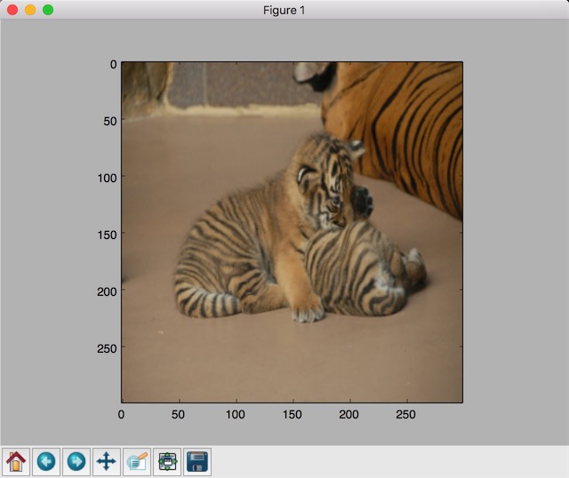
裁剪
croped = tf.image.resize_image_with_crop_or_pad(img_data, 100, 100)
padded = tf.image.resize_image_with_crop_or_pad(img_data, 200, 200)
plt.imshow(croped.eval())
plt.show()
plt.imshow(padded.eval())
plt.show()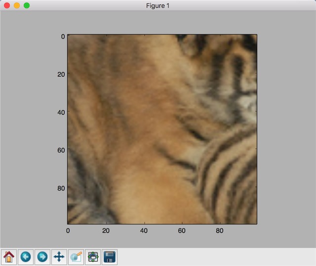
按照一定的比例裁剪:
# 截取中间50%的图片
central_cropped = tf.image.central_crop(img_data, 0.4)
plt.imshow(central_cropped.eval())
plt.show()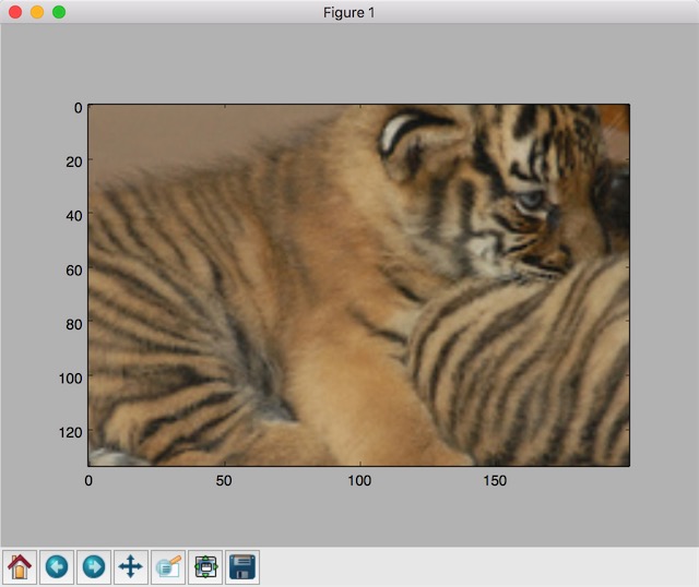
翻转
# 上下翻转
  flipped1 = tf.image.flip_up_down(img_data)
  # 左右翻转
  #flipped2 = tf.image.flip_left_right(img_data)

  #对角线翻转
  # transposed = tf.image.transpose_image(img_data)
  plt.imshow(flipped1.eval())
  plt.show()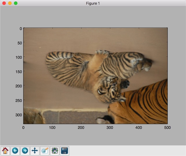
修改亮度、对比度
# 将图片的亮度-0.5。
adjusted = tf.image.adjust_brightness(img_data, -0.5)

# 将图片的亮度+0.5
# adjusted = tf.image.adjust_brightness(img_data, 0.5)

# 在[-max_delta, max_delta)的范围随机调整图片的亮度。
# adjusted = tf.image.random_brightness(img_data, max_delta=0.5)

# 将图片的对比度-5
# adjusted = tf.image.adjust_contrast(img_data, -5)

# 将图片的对比度+5
# adjusted = tf.image.adjust_contrast(img_data, 5)

# 在[lower, upper]的范围随机调整图的对比度。
#adjusted = tf.image.random_contrast(img_data, lower, upper)

# 在最终输出前,将实数取值截取到0-1范围内。
# adjusted = tf.clip_by_value(adjusted, 0.0, 1.0)
plt.imshow(adjusted.eval())
plt.show()
修改色相、
image_float = tf.image.convert_image_dtype(img_data, tf.float32)

adjusted = tf.image.adjust_hue(image_float, 0.1)
# adjusted = tf.image.adjust_hue(image_float, 0.3)
#adjusted = tf.image.adjust_hue(image_float, 0.6)
# adjusted = tf.image.adjust_hue(image_float, 0.9)

# 在[-max_delta, max_delta]的范围随机调整图片的色相。max_delta的取值在[0, 0.5]之间。
#adjusted = tf.image.random_hue(image_float, max_delta)

# 将图片的饱和度-5。
# adjusted = tf.image.adjust_saturation(image_float, -0.1)
# 将图片的饱和度+5。
#adjusted = tf.image.adjust_saturation(image_float, 5)
# 在[lower, upper]的范围随机调整图的饱和度。
#adjusted = tf.image.random_saturation(image_float, lower, upper)

# 将代表一张图片的三维矩阵中的数字均值变为0,方差变为1。
#adjusted = tf.image.per_image_whitening(image_float)

# 在最终输出前,将实数取值截取到0-1范围内。
# adjusted = tf.clip_by_value(adjusted, 0.0, 1.0)
plt.imshow(adjusted.eval())
plt.show()
图片做标记
boxes = tf.constant([[[0.05, 0.05, 0.9, 0.7], [0.35, 0.47, 0.5, 0.56]]])

# sample_distorted_bounding_box要求输入图片必须是实数类型。
image_float = tf.image.convert_image_dtype(img_data, tf.float32)

begin, size, bbox_for_draw = tf.image.sample_distorted_bounding_box(
    tf.shape(image_float), bounding_boxes=boxes, min_object_covered=0.4)

# 截取后的图片
distorted_image = tf.slice(image_float, begin, size)
plt.imshow(distorted_image.eval())
plt.show()

# 在原图上用标注框画出截取的范围。由于原图的分辨率较大(2673x1797),生成的标注框
# 在Jupyter Notebook上通常因边框过细而无法分辨,这里为了演示方便先缩小分辨率。
image_small = tf.image.resize_images(image_float, [180, 267], method=0)
batchced_img = tf.expand_dims(image_small, 0)
image_with_box = tf.image.draw_bounding_boxes(batchced_img, bbox_for_draw)
print(bbox_for_draw.eval())
plt.imshow(image_with_box[0].eval())
plt.show()
对比 PIL 和 TFRecord,我们发现二者虽有很多相同之处,但依旧存在着细微的差别,比如说 PIL 可以做图片合并、Blend 等,甚至基于像素的计算,而 TFRecord 更像是用来对图片做预处理,比如改变图像的大小、打标签等。